Luisen Blog personal blog
Introduction to Genetic Algorithms with C++ to solve TSP

Objective of the post
This post attempts to explain briefly what genetic algorithms are and how and why they help us solve some problems particularly in the field of optimization problems. We will be solving in C++ the classical Travelling Salesman Problem (TSP) using Genetic Algorithms (GA).
A Genetic Algorithms perspective
Genetic algorithms for optimization can be seen as a set of guidelines for designing a heuristic optimization solver in which we trade accuracy in finding the global maxima/minima in return for a faster execution time.
This means that it works as a blueprint algorithm in which every concept or step must be adapted to the problem that is being solved.
An heuristic approach to a simple optimization Problem
This problem will allow us to grasp the main idea in Genetic Algorithms.
Let $f(x) : \mathbb{R} \rightarrow \mathbb{R}$ be a continuous function, we want to find the global maxima of that function in an interval $[a,b]$ with an absolute error of $\epsilon$.
One deterministic way to solve this problem is evaluating for each $x_i = a + i\cdot\epsilon$ the function and update the maximum value found so far, since we do not know future values during the iteration the number of operations required to solve this would be $\frac{b-a}{\epsilon}+1$ considering $\epsilon = 10^{-r}$ this means the number of operations is in the order of $10^r$ leading to a complexity of $O((b-a)\cdot 10^r)$ which can be slow.
Now we will explore a non-deterministic solution, Let $X$ be a set of values $x \in [a,b]$ with cardinal $N$ these values could follow a specific pattern (e.g equally spaced) or could be chosen at random, now evaluate $y_i=f(x_i)$ and keep the $x$(s) that gives the highest value(s), to take advantage of the other points select a point $x’=x_i + (1-\lambda)\cdot (x_{i+1}-x_i) \quad \lambda \in [0,1]$ where $x_i < x_{i+1}$ and evaluate $f(x’)$ update $x_i$ or $x_{i+1}$ according to which gives a higher value. If we iterate this many times and since the $\max_i f(x_i)$ kept is non-decreasing we may end up with a local maxima, global maxima or for some interval $[x_i,x_{i+1}]$ the highest value within a subinterval, to mitigate the possibility of staying at the highest point within an subinterval we could increase the value of $N$ to mitigate the problem of local maxima we could take a random value $x’$ and repeat the process evaluating $f(x’)$ and combining. Since at every step every operation is $O(1)$ and assuming we perform $I$ iterations the total complexity would be $O(IN)$ we can test this algorithm and realize that even for small values of these constants we get a good result, and increasing one or the other yields in a higher accuracy we can increase it until it fulfills our needs “good answer in short time”.
Defining the Genetic Algorithms concepts
The definition of the GA concepts will be described as an analogy to the previuos heuristic solution.
-
Objective Function: Function we want to optmize. In the previous problem this would be $f(x)$
-
Chromosome: A generic variable that our objective function receives. In the previous problem, this would be any $x_i$
-
Population: A set of chromosomes. In the previous example, this would be $X$ with size $N$.
-
Crossover: How we combine chromosomes in hope for better chromosomes. In previuos example this would be $x’=x_i + (1-\lambda)\cdot (x_{i+1}-x_i)$
-
Mutation: A way to avoid staying in local maxima, giving a chance to explore possible better values. In previuos exmaple this would be choosing a random $x$ in hope to improve the maximum value found so far.
this can be easily generalized for functions $f:\mathbb{R}^n\rightarrow\mathbb{R}$
A Biology perspective
So why did we decide to use concepts of biology in optimization problems? Natural selection has shown us that the evolutionary process provides a constant improvement and survival, for a given species a group with less chance to survive will likely not while better suited to current environment will likely do, additionally mutations can either improve the species or not those who do survive in the long term and thus the population benefits. This has happened in animals and particularly human beings the funny thing is that even after a long time, we are not sure we have reached our “global” maxima.
The Travelling Salesman Problem
“Given a list of cities and the distances between each pair of cities, what is the shortest possible route that visits each city and returns to the origin city?”
Brute Force approach
Let the cities be enumerated, we can permute the enumeration of the cities and evaluate the total distance required for the tour of that permutation and store and update the minimal value found in each permutation, of course this leads to a $O(N!)$ which wouldn’t allow to many cities to be considered.
Defining GA variables for the TSP.
-
Objective Function: the total tour distance, we want to minimize this.
-
Chromosome: A particular permutation of the cities.
-
Population: A set of chromosomes.
-
Crossover: We will combine the permutations while preserving the pairs of cities that gives us the shortest distance.
-
Mutation: We will swap the indexes of a permutation and evaluate the objective function of this new permutation.
Implementing the code in C++
First we will define a city as an ordered pair $(x_i, y_i)$ for $i = 0, …,N-1$ in a space $\mathbb{Z}\times\mathbb{Z}$ in a grid $\mbox{NSPACE}\times\mbox{NSPACE}$ we will create 2 arrays one for storing the $x_i$ and another for the $y_i$ (this could also be done with a pair)
Additionally, we will define our main variables NSPACE (grid size), NCities (number of cities), Popul_size (Population size), NIter (Iterations we will run the algorithm) the following values could also be read from a file or user input (stdin).
const int NSPACE = 250;
const int NCities = 15;// 3000;// 15;
const int Popul_size = 12;
const int NIter = 60;
int X[NCities], Y[NCities];
Now we can define our chromosome, this will be defined as a struct with a particular permutation of the cities and the value of the total distance that permutation gives us, which we will name fitness.
struct chromosome{
    int permutation[NCities];
    double fitness;
};
Now we can define our Population as an array of chromosomes:
chromosome Population[Popul_size];
We start by filling the cities with random (we will comment about our randonmess at the end of the post) points within the grid:
srand(time(NULL));
for (int i = 0; i < NCities; i++){
    X[i] = rand() % NSPACE; Y[i] = rand() % NSPACE;
}
Now we initialize our Population with chromosomes with random permutations, to achieve this we will use c++ standard random_shuffle (initialize every permutation ordered from $0$ to $N-1$, then shuffle each permutation)
for (int i = 0; i < Popul_size; i++)
    for (int j = 0; j < NCities; j++)
        Population[i].permutation[j] = j;

for (int i = 0; i < Popul_size; i++)
    random_shuffle(Population[i].permutation, Population[i].permutation + NCities);
Now to evaluate the fitness we will use 2 auxiliary functions:
inline double dist(int u, int v){
    double dx = X[u] - X[v];
    double dy = Y[u] - Y[v];
    return sqrt(dx * dx + dy * dy);
}

double total_dist(int* Cities){
    double total = 0;
    for (int i = 0; i < NCities; i++)
        total += dist(Cities[i], Cities[(i + 1) % NCities]);
    return total;
}
So to evaluate the fitness we only need:
for (int i = 0; i < Popul_size; i++)
    Population[i].fitness = total_dist(Population[i].permutation);
To keep the $\max_i f(P_i)$ where $P_i$ is a particular permutation we can sort the chromosomes and create an auxiliary cmp function for the sorting:
bool cmp(const chromosome& x1, const chromosome& x2){
    return x1.fitness < x2.fitness;
}
To call sort c++ standard library using our cmp function:
sort(Population, Population + Popul_size, cmp);
We can define our mutation function to swap 2 indexes in the permutation, we can also decide to trigger permutation with a chance previously defined, we could also allow or not the mutation if the mutated version is better or not.
void mutate(int* Cities){
    double total1 = 0, total2 = 0;
    total1 = total_dist(Cities);
    int indexA = rand() % NCities, indexB = rand() % NCities;
    swap(Cities[indexA], Cities[indexB]);
    total2 = total_dist(Cities);
    if (total2 > total1 )
        swap(Cities[indexA], Cities[indexB]);
}
Now it’s time to define our principal function of the algorithm, the crossover there can be several ways to define this, in this case, I have chosen the following approach: First we will crossover all the chromosomes only with our best permutation found so far we will evaluate for a particular city which of the 2 chromosomes.permutation give us the shortest distance to the next city in that permutation. (“biologically this means we join and keep the best genes in each of the two chromosomes”) If the next city to be chosen is already chosen we can assign a random city that hasn’t been chosen yet, so our code would be the following:
chromosome crossover(int* p1, int* p2){
    chromosome child;
    bool visited[NCities];
    memset(visited, false, sizeof visited);
    int city = rand() % NCities;
    double dist1, dist2;
    child.permutation[0] = city;
    visited[city] = true;
    int p1x, p2x;
    for (int j = 1; j < NCities; j++){
        for (int i = 0; i < NCities; i++){
            if (city == p1[i]){
                dist1 = dist(p1[i], p1[(i + 1) % NCities]);
                p1x = p1[(i + 1) % NCities];
            }
            if (city == p2[i]){
                dist2 = dist(p2[i], p2[(i + 1) % NCities]);
                p2x = p2[(i + 1) % NCities];
            }
        }
        child.permutation[j] = dist1 < dist2 ? p1x : p2x;
        if (visited[p1x]) child.permutation[j] = p2x;
        else if (!visited[p1x] && visited[p2x]) child.permutation[j] = p1x;
        city = child.permutation[j];
        while (visited[city]){
            city = rand() % NCities;
        }
        child.permutation[j] = city;
        visited[city] = true;
    }
    child.fitness = total_dist(child.permutation);
    return child;
}
Now once we have defined our functions we can code our main loop: for each iteration and for each chromosome we will crossover it with the best chromosome we have so far which will be Population[0] (to keep this as an invariant we will sort the chromosomes) after crossover is performed we will decide to mutate said chromosome with probability Mutate_prob, after each chromosome has followed this procedure we now evaluate its fitness with our total_dist function, then sort the chromosomes so our best value will be Population[0].fitness our code look like this:
for (int iter = 0; iter < NIter; iter++){

    for (int i = 1; i < Popul_size; i++){
        Population[i] =
            crossover(Population[0].permutation, Population[i].permutation);
        int aux = rand() % 100;
        if (aux <= Mutate_prob)
            mutate(Population[i].permutation);
    }

    for (int i = 0; i < Popul_size; i++)
        Population[i].fitness = total_dist(Population[i].permutation);

    sort(Population, Population + Popul_size, cmp);
}
Asymptotic complexity of the code
We need to see the operations we perform in our main loop let $I$ be number of iterations, $N$ the number of cities, $P$ the population size and $C$ the crossover cost.
\[O(IPC + IPN + IP\ln P)\]Evaluating the asymptotic of the crossover function:
$O(N^2 + W)$
Where $W$ is the operations required to evaluate the following code for each city.
while (visited[city]){
    city = rand() % NCities;
}
We will consider the average case complexity.
Let $j$ be the number of cities that have been already visited, let $N$ be the number of cities and $x$ be the city we ask whether we have visited or not, assuming each city to be equally likely to be visited then the probability of x not being visited is: \(P(x) = \frac{N-j}{N}\) Let us define $\lambda$ as our random variable for the number of operations the code results, then we want to determine the expected value of operations i.e $E(\lambda)$ Since we ask “whether x has been visited or not” this behaves as Bernoulli process, this means that The probability that $\lambda = k$ is given by:
\[P(\lambda=k) = \left(\frac{j}{N}\right)^{k-1}\frac{N-j}{N}\]So the expected number of operations is given by:
\[E(\lambda) = \sum \lambda P(\lambda) = \sum_{k=1}^\infty k \left(\frac{j}{N}\right)^{k-1}\frac{N-j}{N}\] \[E(\lambda) = \frac{N-j}{N} \left(\sum_{k=0}^\infty k \left(\frac{j}{N}\right)^{k}+ \sum_{k=0}^\infty \left(\frac{j}{N}\right)^{k}\right)\] \[E(\lambda) = \frac{N-j}{N} \left( \frac{\frac{j}{N} + \left(1 - \frac{j}{N}\right)}{(1-\frac{j}{N})^2} \right)\] \[E(\lambda) = \frac{N}{N-j}\]Which agrees with the expected value of a Bernoulli process with probability $P(x) = \frac{N-j}{N}$
Next we evaluate the total operations for each number of visited cities $j$ ($0$ means no visited cities yet) the total operations would be:
\[\sum_{j=0}^{j=N-1} \left(\frac{N}{N-j}\right) = N \sum_{j=1}^{N} \frac{1}{j} < N \left(1+ \int_{1}^{N} \frac{1}{x} dx \right)\] \[= N(1+\ln N)\]Giving us a total complexity of $W = O(N \ln N)$.
So the total complexity would be $O(IP(N^2 + N \ln N) + IPN + IP\ln P)$ = $O(IPN^2 + IP\ln P)$
If we want to add more cities we could allow a low value for $P$ in which case the complexity would be $O(IPN^2)$. This calculation allow us to prove that our algorithm complexity is far better than the original $O(N!)$ this also allow us to see how we can stress our algorithm.
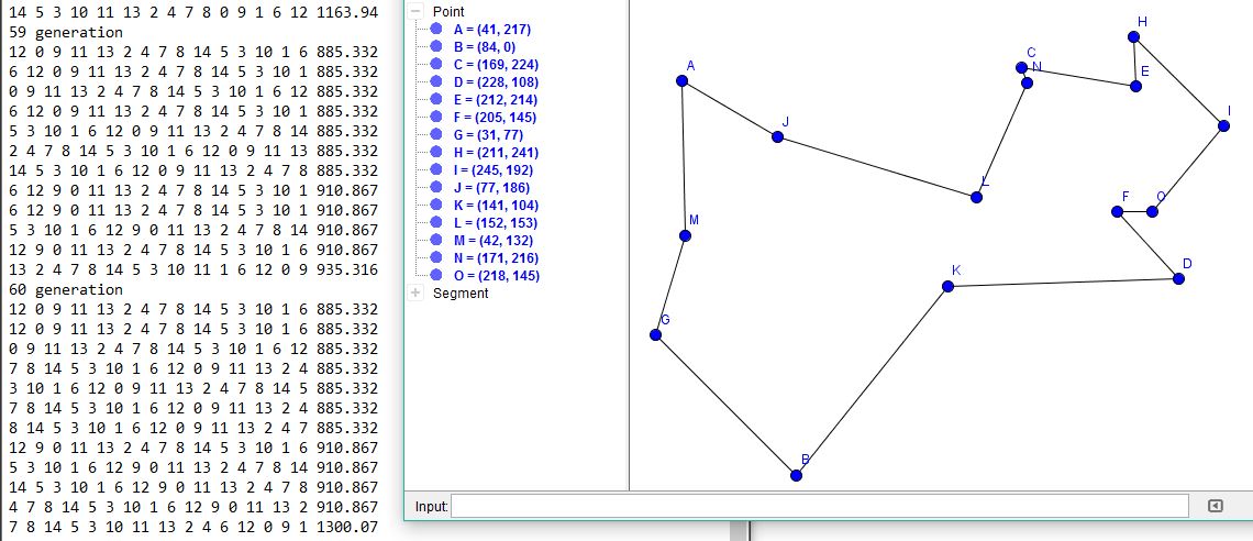
Results